Statistics

[ezcol_1half]

DESCRIPTIVE STATISTICS

• Describe or rank a set of raw data.

[/ezcol_1half]

[ezcol_1half_end]

INFERENTIAL STATISTICS

• Make it possible to know whether the relationships observed in a sample tend to occur in the general population.
• Evaluate the random variability and controls the factors of confusion.

[/ezcol_1half_end]

[ezcol_1half]

MEASURES OF CENTRAL TENDENCY

• Mean.
• Mode.
• Median.
• Confidence interval.

[/ezcol_1half]

[ezcol_1half_end]

MEASURES OF DISPERSION

• Standard deviation.
• Range.
• Variance.

[/ezcol_1half_end]

[ezcol_1half]

EXPERIMENTAL DESIGN

• Searches for differences between two or more sets of data.

[/ezcol_1half]

[ezcol_1half_end]

CORRELATION DESIGN

• Searches for similarities between two or more sets of data.

[/ezcol_1half_end]

WHAT THE STATISTICS SHOULD MEASURE

1st MEAN:

Mean of the population from which the samples are taken.

2nd STANDARD DEVIATION: σ or s

These are measures of the dispersion of the values of the variable in the population and in the sample, respectively.

This is a statistic used as a measure of dispersion or variation in a distribution, equal to the square root of the arithmetic mean of the squares of the deviations from the arithmetic mean.

• Measure of the dispersion of a group of data from its mean. The bigger the difference between the data, the higher the deviation.
• It has the same units as the variable. The standard deviation is invariant with regard to the origin of the distribution.

The standard deviation can also be calculated as the square root of the variation.

3rd CONFIDENCE INTERVAL:

This is a range of values between which the true value of a parameter or the estimation of a series of observations lies.

It enables the precision of the study to be known.

Different samples will lead to different results so a measure of the precision of this estimate is needed, and this is done by calculating the confidence interval (CI= 95%).

A variable cannot be given without its confidence interval, which is what indicates its precision (95% is very good, a 5% error is always left).

4th GOLD STANDARD:

Accepted proof of the standard reference or diagnosis for a specific disease.

5th SENSITIVITY: True positive rate

The probability of the test finding a disease among those who have the disease or the proportion of people with the disease who have a positive test result.

Sensitivity = true positives / (true positives + false negatives)

With reference to a diagnostic test, it is the proportion of truly ill people who have been recorded as such through this test.

6th SPECIFICITY:

This is the probability that the test will NOT find ANY disease among those who do not have the disease or the proportion of people without the disease who have a negative test result.

Specificity = true negatives / (true negatives + false positives)

7th NORMAL DISTRIBUTION: n.

A theoretical frequency distribution for a system of variable data, generally represented by a symmetrical Gaussian bell curve over the mean.

8th CENTRAL TENDENCY:

The centre of a distribution. Described by mean, mid-point and mode.

• Mean: The arithmetic mean in a system of values. The average. It is a measure of centralization for a continuous variable. It is obtained by adding all the sample values and dividing by the sample size.
• Median: For a system of values arranged in order of magnitude, the median is the middle value for the odd numbers of values and the average of the two middle values for an even number of values. In a population or in a sample, it is the value which occupies the central position when all the values are arranged in order from high to low. In a normal distribution, the median corresponds to the 50th percentile. That is, the median means that 50% of the sample values are lower than it and 50% of the sample values are higher than it.
• Mode: For a system of values, in a population it is the most frequent value in a series of observations. It is the value which is most often repeated in a nominal variable.

9th INCIDENCE:

The incidence reflects the number of new “cases” in a period of time.

It is a dynamic index which requires monitoring the population of interest over time.

It can be measured with two indices: accumulated incidence and density (or rate) of incidence.

The accumulated incidence is the proportion of individuals who develop the event during the period of monitoring.

Rate of incidence.

Number of new cases of a disease or other events during a certain period of time, divided by the number of people exposed to the risk during this period.

10th PREVALANCE:

This is the proportion of individuals of a population presenting the event at a certain time, or during a certain period of time. Number of cases of a disease in a given population and at a given time.

For example, the prevalence of diabetes in Madrid in 2001 is the proportion of individuals of that province who in 2001 suffered from the disease.

Rate of prevalence.

Total number of individuals who present an attribute or suffer from a disease at a given time or during a given period of time, divided by the population at risk of having the attribute or the disease at that time or in the middle of the period considered.

11th VARIANCE:

Measures the dispersion of the variable around the mean.

Expected value or expectation or mean.

Measure of the variation of a series of observations; it is equal to the sum of the squares of the deviations with respect to the mean, divided by the number of degrees of freedom of the series. Its square root is the standard deviation.

12th AMPLITUDE OR RANGE:

The difference between the maximum value (this is a sample value such that there are no sample values over and above it) and the minimum value (this is a sample value such that there are no sample values under it) of the values of a variable.

100% of the sample values are found within the amplitude of a variable.

Difference between the maximum and minimum value of a sample or a population. It is only valid in continuous variables.

13th MEASURE OF THE DISPERSION OF A SAMPLE:
This is the positive square root of the variance.

If the sample consists of n values of a variable y, that is, , the standard deviation of y in the sample will be: 

where y is the mean of the sample. 68.3% of the observations are included between standard deviations -1 and +1; 95.4% between -2 and +2, and practically 99.7% between -3 and +3; therefore, in a normal distribution it is expected that only 0.3% of the observations carried out will differ from the mean in more than three standard deviations.

14th STATISTICALLY SIGNIFICANT DIFFERENCES:

The differences between what is observed and what is assumed in the null hypothesis cannot be explained by chance.

15th BIMODAL DISTRIBUTION:

Frequency distribution with two zones of frequency density (which determine two modes) separated by an intermediate zone of low frequency of observations.

16th BINOMIAL DISTRIBUTION:

Distribution of the probability of observing x events in the course of n independent observations in which, in each observation, a probability p identical to the appearance of the event is assumed.

The result of each test should be dichotomous, that is, with two possibilities which mutually exclude each other (for example, presence or absence of disease).

17th FACTORIAL DESIGN:

Design applied in trials in which two or more treatments are tested separately or together, so that interactions between them can be measured.

If the trial includes two drugs or therapeutic interventions A and B, four groups are formed: one treated with A and placebo of B, another one treated with B and placebo of A, another treated simultaneously with A and B and another one treated with placebo A + placebo B.

18th FREQUENCY DISTRIBUTION:

Graph or table showing the frequency with which a value or characteristic occurs in a population or sample according to categories or sub-groups.

Its general position in a scale is described with a measure of central tendency. There are three measures of central tendency: the mean, the median and the mode.

The standard deviation gives information about the dispersion of the value measured in the population studied.

19th POISSON DISTRIBUTION:

Distribution of the probability of observing x episodes of an event when m are expected in a given period.

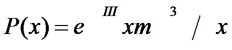
The Poisson distribution derives from the binomial distribution when the number n of observations tends to infinity (in practice, when it is higher than 100) and the probability (which is assumed to be constant in each observation) of the appearance of the event P tends to zero.

The Poisson distribution is often used in pharmacovigilance and pharmacoepidemiology when studying low risks in populations of more than 100 subjects, in order to calculate the probability of appearance of a certain event, calculate the confidence interval of a rate, estimate the number of individuals who should be included in a study, etc.

20th NORMAL OR GAUSSIAN DISTRIBUTION:

It is a theoretical distribution of probability which is used both in theoretical and applied statistics.

It appears in practice frequently as a consequence of the important result which the central limit theorem establishes.

It has a bell-like shape, and is characterised by just two values: the mean and the variance.

Continuous, symmetrical frequency distribution, with two tails which extend to infinity, in which the mean, the median and the mode have the same value and whose shape is determined by the mean and the standard deviation.

21st META-ANALYSIS:

Structured and systematic integration of the information obtained in different studies about a certain problem.

Consists of identifying and reviewing the controlled studies about a specific problem, in order to give a summarized quantitative estimate of all the available studies.

Given that it includes a greater number of observations, a meta-analysis has greater statistical power than the clinical trials it includes.

The two main methodological problems of the meta-analysis of clinical trials are:

• the heterogeneity among the trials included (in terms of clinical and socio-demographic characteristics of the populations included in each trial, the clinical evaluation methods applied, the dose, the pharmaceutical form or dosage guidelines of the drug evaluated, etc.).
• the possible bias of publication (derived from the fact that not all clinical trials actually carried out have been published).

22nd LINEAR MODEL:

Statistical model in which the value of a parameter y is equal to a + bx, where a (rank ordered in the origin) and b (slope, the value of which is found between -1 and +1) are constant.

23rd LOGISTIC MODEL:

Statistical model of probability of the disease y according to a risk factor x, in which where P (y/x) is the probability that y will appear among the subjects exposed to the factor x and e is the natural exponential function.

In the multiple logistic model, the fixed term is substituted for a linear term which includes various factors, for example:  if two factors x1 and x2 exist.

24th LEVEL OF SIGNIFICANCE:

In statistical significance tests, it is the value of p, which, in the strictest sense, in a clinical trial should be pre-specified in the design phase.

The most frequently accepted level is 0.05, but levels of 0.01, 0.001 etc, may also be applied.

25th NUMBER NEEDED TO TREAT (NNT):

When the experimental treatment increases the probability of a favourable event (or when it reduces that of an adverse event), the number of patients which need to be treated to give rise to another patient with improvement (or to prevent an additional adverse event).

It is calculated as 1/RAR, rounded up to the next immediate integer, along with a confidence interval of 95%.

26th P (p- value):

The level of significance observed in the test.

The smaller it is, the greater the evidence to reject the null hypothesis.

27th P (PROBABILITY):

Followed by the abbreviation n.s. (not significant) or the symbol < (less than) and a decimal number (for example, 0.05 or 0.01), it indicates the probability that the difference observed in a sample has occurred purely by chance, the groups compared really being similar, that is, under the null hypothesis.

28th PERCENTILE:

A 90th percentile corresponds to a value which divides the sample into two parts, so that 90% of the sample values are lower than this vale, and 10% of the sample values are higher than this value.

The 25th, 50th and 75th percentiles are the first, second and third quartiles respectively.

In a series (sufficiently big) of ordered observations (for example, ranked from smallest to biggest), the part which constitutes a certain percentage of all the elements in the series.

For example, in a series of height values (in cm), the first decile will be made up of the weights of the 10% containing the smallest individuals, and the tenth decile will be made up of the 10% containing the tallest subjects.

Similarly, the first quartile or the first quintile will consist, respectively, of 25% and 20% of the smallest individuals.

In a normal distribution, the median is exactly equivalent to the 50th percentile (50% of the individuals are over and 50% are below the median).

29th CORRELATION COEFFICIENT:

Measure of association which indicates the extent to which two continuous variables x and y have a linear relationship (y = a ± bx).

It is designated with the letter r, and its value can be between -1 and +1.

The values -1 and +1 – indicate that there is a perfect linear relationship, negative or positive respectively, between both variables, and when represented on coordinate axes, the data is distributed in a straight line, with a negative or positive slope, respectively.

When r = 0, the data is arranged in a circle and there is no degree of correlation.

30th COEFFICIENT OF VARIATION:

Standard deviation expressed as a percentage of the mean, that is, (DE/x) X 100.

31st CLINICAL SIGNIFICANCE:

Probability that an observed difference has a repercussion on the course of the problem or disease treated that is relevant for a given patient or for a group of patients.

It should not be confused with the statistical significance: there are often descriptions of statistically significant differences which are not clinically significant.

32nd STATISTICAL SIGNIFICANCE:

Probability that an observed difference is the result of chance and not the causal determinants in the study.

The finding of a statistical significance does not necessarily imply clinical significance.

33rd CONTINGENCY TABLE:

A table of 2 or more variables, where the individuals which belong to each combination of the possible levels of these variables are entered in each cell.
Tabular classification of data of a population sample, in which the sub-categories of a characteristic are entered horizontally (in rows) and those of the other characteristic are entered vertically (in columns).

Tests of association can thus be applied between the characteristics of the rows and those of the columns.

The simplest contingency table is a 2 x 2 one, which includes two categories of the characteristic in the rows and two categories of the characteristic in the columns (that is, four values).

To examine the results of a clinical trial, data referring to the experimental group is usually put in the upper row and that corresponding to the reference group in the lower row.

The number of patients who present the studied event is usually put in the first column and the number of those who do not present the event is put in the second column.